Wednesday 21 September 2011

Variogram fit with RPanel

During the UseR 2011 conference I saw lots of examples of the use of RPanel to create a GUI in R. Yesterday, because I was a bit bored of the work I was doing I started thinking about this and I decided to try this package.

My objective was to create a new panel with all the main setting for fitting a variogram model to an omnidirectional variogram with gstat.

This is the script:

library(rpanel)
library(gstat)

data<-read.table("data.txt",sep="",header=T)
coordinates(data)=~Lat+Lon

##Variogram Fitting
variogram.plot <- function(panel) {
with(panel, {
variogram<-variogram(Oxigen~1,data,cutoff=Cutoff)
vgm.var<-vgm(psill=Sill,model=Model,range=Range,nugget=Nugget)
#fit<-fit.variogram(variogram,vgm.var)
plot(variogram$dist,variogram$gamma,xlab="Distance",ylab="Semivariance")
lines(variogramLine(vgm.var,maxdist=Range))
})
panel
}

var.panel <- rp.control("Variogram",Sill=20,Range=250,Nugget=0,Model="Mat",Cutoff=250)
rp.listbox(var.panel,Model,c("Mat","Sph","Gau"))
rp.slider(var.panel, Cutoff, 0,500,showvalue=T)
rp.slider(var.panel, Sill, 0,500,showvalue=T)
rp.slider(var.panel, Range, 0,1000,showvalue=T)
rp.slider(var.panel, Nugget, 0,15,showvalue=T)
rp.button(var.panel, title = "Fit", action = variogram.plot)


At this address you can find a zip file with a sample dataset that you can use to try this script, however if you know a bit of gstat you can start customizing it straigth away:


This is the screenshot from my R Console:
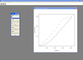


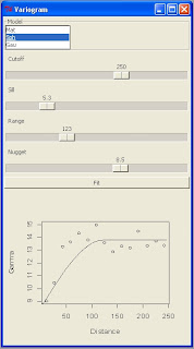
I also tried to embed the variogram plot into the panel in order to execute the script in batch mode, this is the result:


if(print(require(tcltk))==FALSE){install.packages("tcltk",repos="http://cran.r-project.org")}
if(print(require(tcltk))==TRUE){require(tcltk)}

if(print(require(rpanel))==FALSE){install.packages("rpanel",repos="http://cran.r-project.org")}
if(print(require(rpanel))==TRUE){require(rpanel)}

if(print(require(gstat))==FALSE){install.packages("gstat",repos="http://cran.r-project.org")}
if(print(require(gstat))==TRUE){require(gstat)}


data<-read.table(tclvalue(tkgetOpenFile()),sep="",header=T)
coordinates(data)=~Lat+Lon

grid <- spsample(data, cellsize = 10, type = "regular")
gridded(grid) <- TRUE


##Variogram Fitting
variogram.plot <- function(panel) {
with(panel, {
variogram<-variogram(Oxigen~1,data,cutoff=Cutoff)
vgm.var<-vgm(psill=Sill,model=Model,range=Range,nugget=Nugget)
#fit<-fit.variogram(variogram,vgm.var)
plot(variogram$dist,variogram$gamma,xlab="Distance",ylab="Gamma")
lines(variogramLine(vgm.var,maxdist=Range*2))
})
panel
}

replot.smooth <- function(object) {
rp.tkrreplot(var.panel, plot)
object
}


var.panel <- rp.control("Variogram",Sill=20,Range=250,Nugget=0,Model="Mat",Cutoff=250,size=c(800,600))
rp.listbox(var.panel,Model,c("Mat","Sph","Gau"))
rp.slider(var.panel, Cutoff, 0,sqrt(areaSpatialGrid(grid)),showvalue=T)
rp.slider(var.panel, Sill, 0,var(data$Oxigen)*2,showvalue=T)
rp.slider(var.panel, Range, 0,sqrt(areaSpatialGrid(grid)),showvalue=T)
rp.slider(var.panel, Nugget, 0,var(data$Oxigen),showvalue=T)
rp.button(var.panel, title = "Fit",action=replot.smooth)
rp.tkrplot(var.panel, plot,variogram.plot)
rp.block(var.panel)


It probably need some more work in order to be perfect but at the moment I'm not interested in a perfect automatic script.
If someone has time to spend on it and is able to made it perfectly automatic for every data file, please share the script with the community.

By the way, I also implemented a line from the tcltk package for the selection of the data file interactively.
This is the resulting panel:
Wednesday 13 April 2011

CoKriging with gstat - Videotutorial

This is the last lesson of the R Videotutorial for spatial statistics.
It is all about cokriging in gstat. For this lesson I used the meuse dataset, available within gstat, for the references to this dataset take a look at the script.

The videotutorial is available at this link:
Lesson 6

The script and the dataset for the lesson are available here:
Script


P.S.
Thanks to Gerald that with his email remembered me about this lesson, which I uploaded to the site several days ago but I forgot to mentioned in the blog.

Tuesday 12 April 2011

Box Plot with ggplot2

Hi,
in these days I'm creating lots and lots of box plot with ggplot2.
The look of them is really good and you can change every bit of code so that you can customize the plot completely.
Here is the code I'm using with a test data file to try it:
BoxPlot.zip

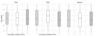
The result looks like this:

Wednesday 16 March 2011

Textural triangle plot in R

Hi,
these days I'm working with soil textural data and one of the key point of these data is the presentation of the results.
The best way is a old-school texture triangle!!!

Because I like to do all my stuff in R, instead of opening draw software such as corel draw or adobe illustrator, I started looking at packages for this kind of plot.

I think the best one is plotrix, because it let's you plot the USDA or UK textura triangle, so in the end the image is ready for publication.

I prepared a little script to show how to create a simple plot, adding the legend and save it as image file.
The script is downloadable from this link:
R script

I'm also preparing a little video for showing how to use the script but if you are familiar with R, you don't need it.

Friday 11 March 2011

Script for Geostatistics with R

I received requests for the script used during the tutorial.
All the material is available in the main page of the course.
However, in order to facilitate the availability of the scripts to all the viewers of this blog I've put the link to donwnload them at the end of this post.

This zip file contains 3 R scripts:
- Lesson3: How to handle and plot spatial data in R
- Lesson4: How to perform an Ordinary Kriging with gstat
- Lesson5: How to perform a Universal Kriging with gstat

And here is the link:
R script

Thursday 3 March 2011

3D Anisotropy parameters

Hello everyone,

I’m trying to create a method for calculating the 5 parameters for the 3D anisotropy in an automatic way.

Basically I created a loop for analysing the range of the horizontal variogram in every direction and extrapolating the maximum (for the angle p). Then it computes the vertical variogram in the direction of maximum continuity and extrapolates the maximum range (for the angle q).

Subsequently, it computes the vertical variogram for the direction of minimum continuity (angle of max continuity + 90), and extrapolates the maximum (for the angle r).

Ultimately, it calculates the ratio between the range of the maximum continuity and the other 2.

I would like to know what the community think of this idea.

Could you please tell me if it makes sense and, if it does, how to improve it?

So far I wrote the following lines:

library(gstat, pos=4)

library(sp, pos=4)

library(lattice)

c1<-read.asciigrid("dtm.asc")

##a covariate that will be used to specify the cutoff of the variogram

data<-read.table("data.txt",sep="",header=T)

##Data format:

## Lat = latitude

## Lon = longitude

## depth = depth

## value = data value

coordinates(data)=~Lat+Lon+depth

##Anisotropy

##First Loop for angle p

mod<-vgm(var(data$value),"Sph",sqrt(areaSpatialGrid(c1)),0)

write.table(matrix(c("Angle","Range"),ncol=2),"hor.txt",col.names=F,row.names=F)

for(i in 0:180){

angl<-as.data.frame(fit.variogram(variogram(value~1,data,cutoff=sqrt(areaSpatialGrid(c1)),width=sqrt(areaSpatialGrid(c1))/15,alpha=c(i),tol.hor=10),mod,fit.method=6))[2,3]

write.table(matrix(c(i,angl),ncol=2),"hor.txt",append=T,row.names=F,col.names=F)}

hor<-read.table("hor.txt",sep="",header=T)

xyplot(Range~Angle,data=hor,type="l",xlim=0:180,scales=list(x=list(tick.number=15),tck=0.5))

max_range<-subset(hor,hor$Range==max(hor$Range))

##Second Loop for angle q

mod_depth<-vgm(var(data$value),"Mat",max((data@coords)[,3]),0)

write.table(matrix(c("Angle","Range"),ncol=2),"ver1.txt",col.names=F,row.names=F)

for(i in 0:180){

angl<-as.data.frame(fit.variogram(variogram(value~1,data,cutoff=max((data@coords)[,3]),width=max((data@coords)[,3])/length((data@coords)[,3]),alpha=c(max(max_range$Angle)),beta=c(i),tol.hor=10,tol.ver=10),mod_depth,fit.method=6))[2,3]

write.table(matrix(c(i,angl),ncol=2),"ver1.txt",append=T,row.names=F,col.names=F)}

ver1<-read.table("ver1.txt",sep="",header=T)

xyplot(Range~Angle,data=ver1,type="l",xlim=0:180,scales=list(x=list(tick.number=15),tck=0.5))

max_range1<-subset(ver1,ver1$Range==max(ver1$Range))

##Third Loop for angle r

mod_depth<-vgm(var(data$value),"Mat",max((data@coords)[,3]),0)

write.table(matrix(c("Angle","Range"),ncol=2),"ver2.txt",col.names=F,row.names=F)

for(i in 0:180){

angl<-as.data.frame(fit.variogram(variogram(value~1,data,cutoff=max((data@coords)[,3]),width=max((data@coords)[,3])/length((data@coords)[,3]),alpha=c(max(max_range$Angle)+90),beta=c(i),tol.hor=10,tol.ver=10),mod_depth,fit.method=6))[2,3]

write.table(matrix(c(i,angl),ncol=2),"ver2.txt",append=T,row.names=F,col.names=F)}

ver2<-read.table("ver2.txt",sep="",header=T)

xyplot(Range~Angle,data=ver2,type="l",xlim=0:180,scales=list(x=list(tick.number=15),tck=0.5))

max_range2<-subset(ver2,ver2$Range==max(ver2$Range))

##Parameters

p=max(max_range$Angle)

q=max(max_range1$Angle)

r=max(max_range2$Angle)

s=max(max_range$Range)/max(max_range1$Range)

t=max(max_range$Range)/max(max_range2$Range)

R Video Tutorial for Spatial Statistics

Welcome everybody, this is a video tutorial that will try to teach you how to use R for spatial statistics and interpolation.

I’m a PhD student in soil science and in particular my project is about digital soil mapping. During my work I often use R particularly for geostatstical interpolation. Despite R being a very powerful statistical language which has became a benchmark for spatial statistics, it is also a relatively difficult language to learn with one of the steepest learning curve among programming languages.

For this reason I though about sharing what I’ve learned during my PhD with all the R community. I prepared this video tutorial because I think that the easy way of learning R is by examples.

The tutorial is structured as follow: the first two lesson are about the basics of R, how to handle R objects, plotting and saving your work. This part is intended for a beginner user who want to learn the language. Starting from the third lesson I will show examples on how to handle and plotting spatial data and rasters, and in the last two lesson I will show you how to perform an ordinary and a universal kriging in R.

In this tutorial I will show you some example that will hopefully help you learning R in a quicker and easier way. However, this course is not a complete R course, because R has lots and lots of different functions for every branch of science. For this reason at the beginning of the course and at the end of the lesson, if appropriate, I will give you some references if you want to deepen your knowledge.

The link to the course is here: http://www.fabioveronesi.net/rtutorial.html


If you have any suggestion at all on how to improve the course or any other feedback, send an e-mail to: r-course@fabioveronesi.net